40 conditional formatting data labels excel

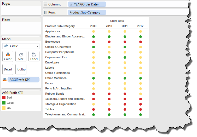
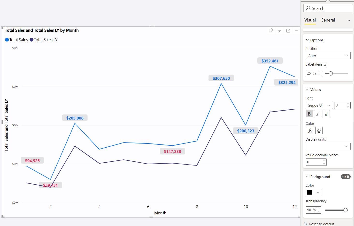
Power BI September 2022 Feature Summary Conditional formatting for data labels. Last month, we released an update to conditional formatting for data labels to have them apply to each individual data point rather than all of them together. At the time, this improvement was limited to visuals without a field in the Legend field well. Charts and Dashboards: Conditional Chart Labelling - Part 1 I will address all four areas, as I try to create the appearance of conditional formatting, but this week I will concentrate on step 1. Step 1: Creating Multiple Number Formats in Excel This is more a challenge of understanding how it works, rather than trying to solve the problem from scratch, as the inputs have already been formatted accordingly.

How to Print Avery Labels from Excel (2 Simple Methods) - ExcelDemy Following, navigate to Mailings > Start Mail Merge > Labels. Now, choose the options as shown in the image below and click OK to close the dialog box. Next, select Design > Page Borders. Immediately, a Wizard box appears, choose Borders > Grid. This generates the grid in the blank document. Step 03: Import Recipient List From Excel into Word

Conditional formatting data labels excel

How to change chart axis labels' font color and size in Excel? Apply conditional formatting to fill columns in a chart. By default, all data point in one data series are filled with same color. Here, with the Color Chart by Value tool of Kutools for Excel, you can easily apply conditional formatting to a chart, and fill data points with different colors based on point values. Full Feature Free Trial 30-day! How to use Conditional Formatting in Excel to Color-Code ... - LaptopMag 3. Choose Conditional Formatting from the ribbon. 5. We're going to color-code bills that we haven't paid. To do that, add "NO" to the Format cells that are EQUAL TO box, and then select a color... Conditional formatting one cell - Microsoft Tech Community Conditional formatting one cell I am using Excel in Microsoft 365. I want to conditionally format a single standalone cell (not a range of cells) to turn light red with dark red text when that cell has a value of less than or equal to 80 entered. Everything I find talks about a range of cells. I am looking for just one single cell.

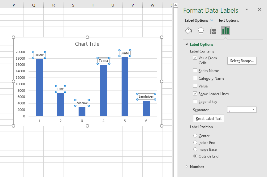
Conditional formatting data labels excel. Conditional Formatting Shapes - Step by step Tutorial Enter 1 in both cells. As an effect of the conditional formatting, both cells will turn green, so the rule we have set before will prevail. We can control the shape with the change in the cell's value. This was, in any case, the simplest solution for the use of Conditional Formatting on a shape. Progress Doughnut Chart with Conditional Formatting in Excel 24.03.2017 · Great question! The Excel Web App does not support those text box shapes yet. We can use the built-in data labels for the chart instead. The label for the Remainder bar can be deleted by left clicking on the label twice, then pressing the delete key. That just leaves the data label for the actual progress amount. Here is a screenshot. How to do Conditional Formatting on Stacked Bar Chart in Excel Then, drag down to copy the formula to the entire column and type "0" in the blank cells. 2. Second, input the formula "=IF (B2<100;B2;"")" in cell C9. Similarly, drag down to copy and type "0" in the blank cells. 3. Third, select A9:C13. Click to Insert and go to the Charts. From there, select the Stacked Column. chandoo.org › wp › change-data-labels-in-chartsHow to Change Excel Chart Data Labels to Custom Values? May 05, 2010 · Now, click on any data label. This will select “all” data labels. Now click once again. At this point excel will select only one data label. Go to Formula bar, press = and point to the cell where the data label for that chart data point is defined. Repeat the process for all other data labels, one after another. See the screencast.

Custom data label color based on another cell Value (Priority) Windows. Feb 11, 2022. #2. You can do this, by using conditional formatting (just as you maybe have other places in the Gantt Chart). Mark the area you will use, and in conditional format choose, "New rule" and insert: IF (A$1=1;TRUE). A1 has to reflect the cell you have the value in, and 1 in the formula, are the value you will use. Up and Down Arrows in Excel conditional formatting Select a cell Select the first cell of the data to which you want to apply conditional formatting. Select a range Press Shift + ↓ (Down Arrow key) to select multiple cells. Select an arrow from the icon set Press Alt + H + L + I (ai), then press Enter. Up and down arrows applied to data The arrow has been applied to the data. › pivot-tables › pivot-tableHow to Apply Conditional Formatting to Pivot Tables - Excel ... Dec 13, 2018 · Conditional Formatting can change the font, fill, and border colors of cells. It can also add icons and data bars to the cells. The formatting will also be applied when the values of cells change. This is great for interactive pivot tables where the values might change based on a filter or slicer. How to Setup Conditional Formatting for Pivot ... Excel Conditional Formatting not functioning correctly after … 10.01.2018 · Everything works fine, formatting changes according to changes in the data! Now I copy a range of sheet A to sheet B using VBA, that works OK. However: in sheet B the conditional formatting of these cells is not working correctly anymore: > cells using 'format only cells that contain' work correct! formatting changes correctly when data changes

› conditional-formatting-for-blankConditional Formatting For Blank Cells | (Examples and Excel ... Always use limited data to deal with and apply bigger conditional formatting to avoid excel getting freeze. Recommended Articles. This has been a guide to Conditional Formatting for Blank Cells. Here we discuss how to apply Conditional formatting for blank cells along with practical examples and a downloadable excel template. › data-bars-in-excelHow to Add Data Bars in Excel? - EDUCBA How to Add Data Bars in Excel? Data Bars in Excel. Data Bars in Excel is the combination of Data and Bar Chart inside the cell, which shows the percentage of selected data or where the selected value rests on the bars inside the cell. Data bar can be accessed from the Home menu ribbon’s Conditional formatting option’ drop-down list. techcommunity.microsoft.com › t5 › excel-blogMicrosoft Excel conditional number formatting Sep 17, 2019 · Next, I would apply conditional formatting number formatting where the cell value is greater than one so that numbers greater than a million could be displayed to the nearest 0.1m, numbers less than a million but greater than or equal to 1,000 could be displayed to the nearest 0.00k and numbers lower than 1,000 (but necessarily greater than one ... How to Copy Conditional Formatting in Microsoft Excel Open the tool by going to the Home tab and clicking the Conditional Formatting drop-down arrow. Select "Manage Rules." When the Conditional Formatting Rules Manager opens, select "This Worksheet" in the drop-down box at the top. If the rule you want to duplicate is on a different sheet, you can select it from the drop-down list instead.

CIS Ch3 Excel Flashcards | Quizlet

Conditional formatting shortcut - Excel Hack Press Alt + H + L + S to display a menu where you can select the color scales. Use the Arrow keys, etc. to select the color of your choice. The color scale has been applied to the cells. Display the Conditional Formatting Rules Manager dialog box Select a cell. Press Alt + O + D or Alt + H + L + R.

How to improve or conditionally format data labels in Power ...

How to change cell formatting using a Drop Down list - Get Digital Help Select cell D3. Go to tab "Data" on the ribbon. Press with left mouse button on "Data Validation" button on the ribbon and a dialog box appears. Go to tab "Settings" on the dialog box. See image below. Select List. Type: No formatting, %, Time, Above Average, Below Average.

Conditional Formatting

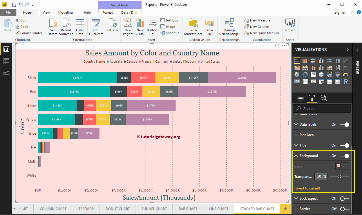
Conditional Formatting Using Custom Measure - Power BI 28.09.2020 · Voila! We have given conditional formatting to Day of Week column based on the clothing Category value. I just tried to add a simple legend on the top to represent the color coding. So, this is how one can use a custom color formatting in Power BI by creating a simple measure for it. Hope this article helps everyone out there. - Pragati

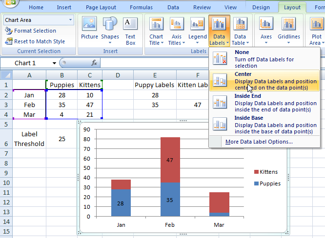
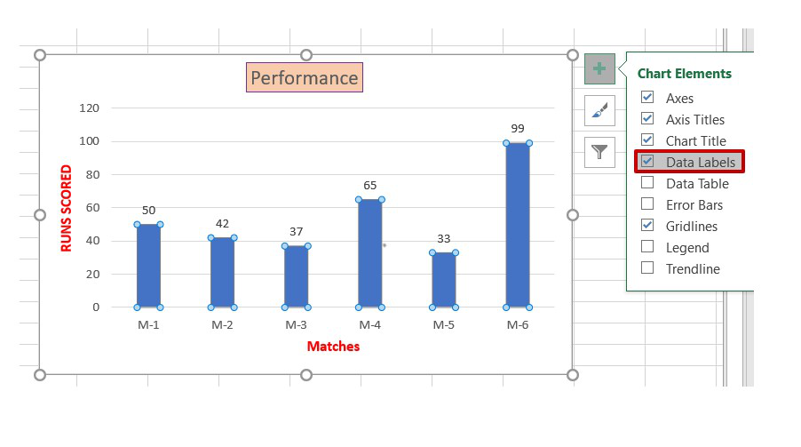
Adding Data Labels To An Excel Chart | MyExcelOnline

Easy Conditional Mail Merge Formatting (If...Then...Else): MS … 08.12.2021 · 13. If you want to apply conditional formatting manually, you need to use Ctrl+F9 to add the curly braces and the field codes. Note: Don’t use spaces in your field names. Formatting the Conditional Text in Word Mail Merge. When you perform a merge mail in Microsoft Word, the formatting of an MS Excel data file is lost. You must edit the field ...

Custom Data Labels with Colors and Symbols in Excel Charts ...

A Quick Guide to Conditional Formatting in Excel - HubSpot The image below is the sample data set I'll use for this explanation: 1. First, select column B. 2. Navigate to the header toolbar and select Conditional Formatting. When the Conditional Formatting drop-down menu appears, select Highlight Cells Rules, then Equal To. 3. In the New Formatting dialog box, select Cell Value and Equal To.

Example: Charts with Data Labels — XlsxWriter Documentation

How to Apply Conditional Formatting to Pivot Tables - Excel … 13.12.2018 · Conditional Formatting can change the font, fill, and border colors of cells. It can also add icons and data bars to the cells. The formatting will also be applied when the values of cells change. This is great for interactive pivot tables where the values might change based on a filter or slicer. How to Setup Conditional Formatting for Pivot ...

Excel - Beyond the Basics Part Two: Using Conditional ...

Custom Chart Data Labels In Excel With Formulas - How To Excel At Excel Follow the steps below to create the custom data labels. Select the chart label you want to change. In the formula-bar hit = (equals), select the cell reference containing your chart label's data. In this case, the first label is in cell E2. Finally, repeat for all your chart laebls.

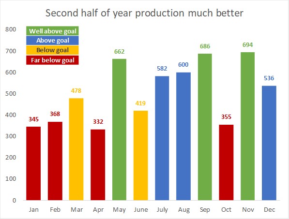
Conditional formatting for Excel column charts | Think ...

Microsoft Excel conditional number formatting 17.09.2019 · Next, I would apply conditional formatting number formatting where the cell value is greater than one so that numbers greater than a million could be displayed to the nearest 0.1m, numbers less than a million but greater than or equal to 1,000 could be displayed to the nearest 0.00k and numbers lower than 1,000 (but necessarily greater than one) could be displayed as …

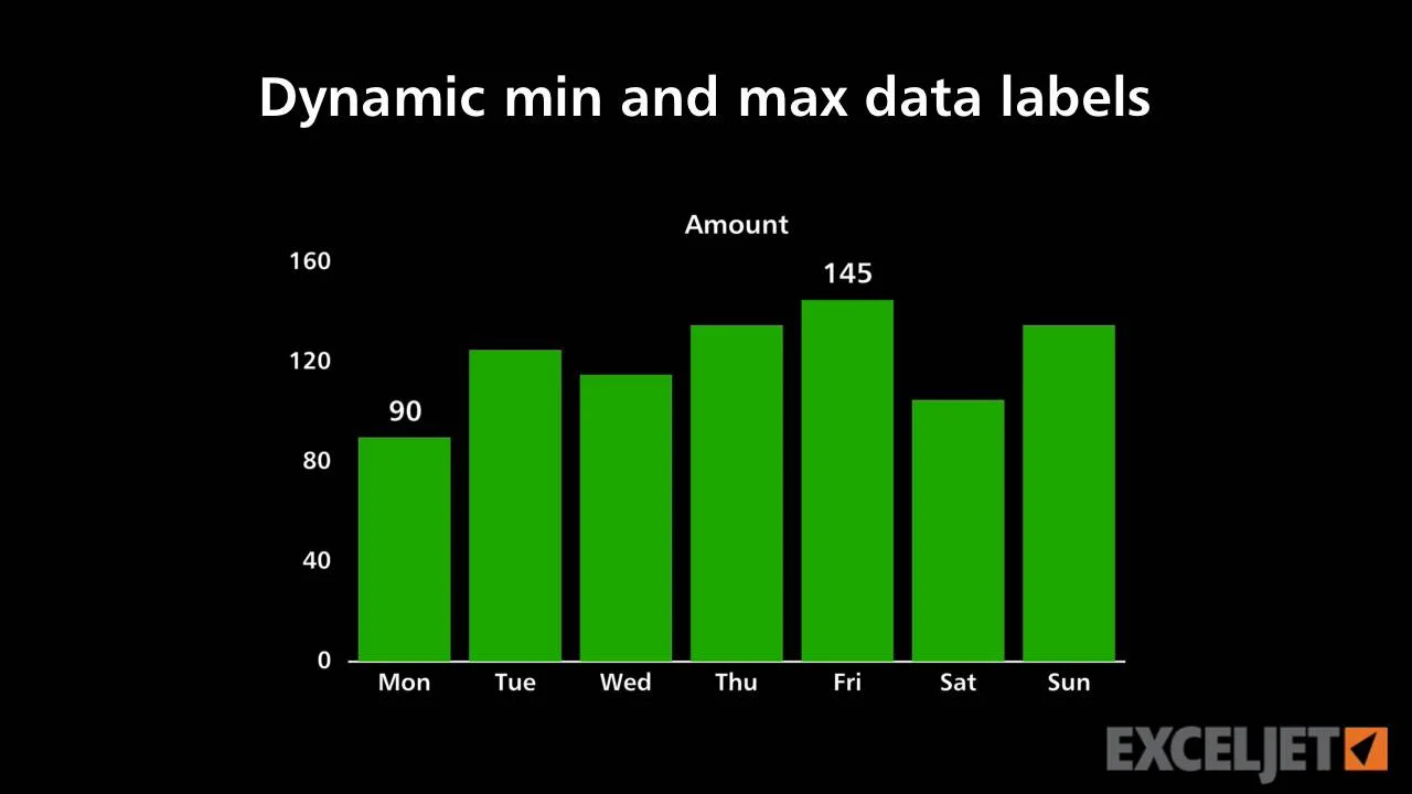
Dynamic min and max data labels

How to Use Conditional Formatting in Excel (Step-by-Step) Locate the conditional formatting button. Once you select your data, the next step is to locate the conditional formatting button. Locate the "Home" tab and click on the "Styles" group. Excel separates each group with a vertical line and labels them at the bottom. Finally, click on "Conditional Formatting."

Is it possible to conditionally format Data Labels on a ...

Conditional Formatting For Blank Cells - EDUCBA Always use limited data to deal with and apply bigger conditional formatting to avoid excel getting freeze. Recommended Articles. This has been a guide to Conditional Formatting for Blank Cells. Here we discuss how to apply Conditional formatting for blank cells along with practical examples and a downloadable excel template. You can also go ...

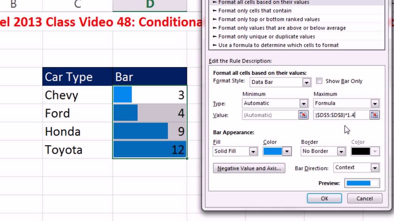
Highline Excel 2013 Class Video 48: Conditional Formatting: Bar Chart with Data Labels

techcommunity.microsoft.com › t5 › excelExcel Conditional Formatting not functioning correctly after ... Jan 10, 2018 · Everything works fine, formatting changes according to changes in the data! Now I copy a range of sheet A to sheet B using VBA, that works OK. However: in sheet B the conditional formatting of these cells is not working correctly anymore: > cells using 'format only cells that contain' work correct! formatting changes correctly when data changes

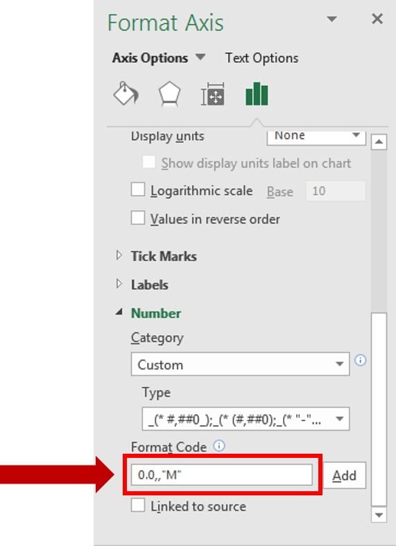
Dynamic Number Format for Millions and Thousands - PK: An ...

Conditional Formatting with Data Validation - Microsoft Tech Community Select the range in column C that you want to format, for example C2:C100. The first cell in the range (C2 in this example) should be the active cell in the selection. On the Home tab of the ribbon, select Conditional Formatting > New Rule... Select 'Use a formula to determine which cells to format'. Enter the formula

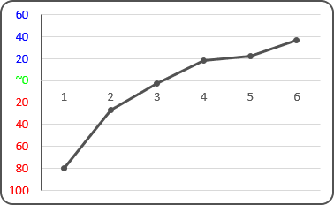
Highlight Max & Min Values in an Excel Line Chart - Xelplus ...

Apply conditional table formatting in Power BI - Power BI To apply conditional formatting, select a Table or Matrix visualization in Power BI Desktop or the Power BI service. In the Visualizations pane, right-click or select the down-arrow next to the field in the Values well that you want to format. Select Conditional formatting, and then select the type of formatting to apply. Note

How to: Display and Format Data Labels | .NET File Format ...

Conditional formatting for Data Labels in Power BI Where you can find the conditional formatting options? Select the visual > Go to the formatting pane> under Data labels > Values > Color Data Labels Let's Get Started- Add one line chart visual into page and create two measure for Profit & Sales. Note: If you don't want to create measure then you can directly use Sales and Profit fields.

How to insert data labels to a Pie chart in Excel 2013

› charts › progProgress Doughnut Chart with Conditional Formatting in Excel Mar 24, 2017 · Great question! The Excel Web App does not support those text box shapes yet. We can use the built-in data labels for the chart instead. The label for the Remainder bar can be deleted by left clicking on the label twice, then pressing the delete key. That just leaves the data label for the actual progress amount. Here is a screenshot.

Improve your X Y Scatter Chart with custom data labels

Change the Font Size, Color, and Style of an Excel Form Control Label So to change the Label's formatting — even when it's linked to the same cell — you'll need to click the label, click the formula bar, and retype the cell link. Admittedly, everyone else might have already figured this one out. However, I'm still very excited.

Apply Custom Data Labels to Charted Points - Peltier Tech

How To Use Conditional Formatting in Excel in 5 Steps Excel separates each group with a vertical line and labels at the bottom of the group. Finally, click on the "Conditional Formatting" button. 4. Select an option from the drop-down menu Once you select the "Conditional Formatting" button, Excel displays several options, starting with "Highlight Cells Rules" and ending with "Manage Rules."

August 2022 Updates for Power BI < News | SumProduct are ...

How To Color Code in Excel Using Conditional Formatting 3. Navigate to Conditional Formatting. Once you've selected all the data you want to format, you can navigate to the "Conditional Formatting" section of Excel. First access the "Home" tab near the top left of the program. Then go to the section labeled "Styles" and select the drop-down menu that says "Conditional Formatting."

How-to Make Conditional Label Values in an Excel Stacked ...

Using Conditional Formatting to Identify Date-Based Patterns in Excel In the New Formatting Rule box, select "Use a formula to determine which cells to format" as the rule type. Choose "Use a formula to determine which cells to format" to set custom date-based formatting. Enter the formula for the dates you want to highlight in the following format: "=TODAY ()-A1>X" where A1 is the cell number of the first cell ...

Align data labels in a graph so they are all along the same ...

Highlight Cell Rules based on date labels | MyExcelOnline One of the most common ways of highlighting. values in pivot tables is by using conditional formatting. Adding conditional formatting. to Pivot Tables can brighten up the data and make it easier to analyze and interpret. Let us see how one can highlight cell rules based on date labels in a pivot table. Download this Excel Workbook and follow ...

Excel Bar Graph Color with Conditional Formatting (3 Suitable ...

How to Apply Different Types of Conditional Formatting in Excel How to Apply Data Bars Conditional Formatting in Excel. The third type of conditional formatting in Excel is Data Bars. So this will create bars in our data set representing both the positive and negative values. And to apply this type of conditional formatting in Excel, let's learn the following steps below: 1. Firstly, select the needed ...

How to change chart axis labels' font color and size in Excel?

Data Bars in Excel (Examples) | How to Add Data Bars in Excel? - EDUCBA Data Bars in Excel is the combination of Data and Bar Chart inside the cell, which shows the percentage of selected data or where the selected value rests on the bars inside the cell. Data bar can be accessed from the Home menu ribbon’s Conditional formatting option’ drop-down list. If we go there, we will be able to see Gradient Fill and Sold Fill Data bar. Whereas gradient …

Conditional Formatting (Fill Color, Font Color etc...) for ...

Excel Conditional formatting on two criteria in a separate table Let's say that if the CustomerID and Period in the data table has the label "Applied" then I want that cell in the top table, where CustomerID and Period intersect, to be coloured RED. If it's "Passed", I want it to be coloured green, and so on. The periods are dates data types. The tables are excel tables.

Adding Data Labels to Your Chart (Microsoft Excel)

How to Print Avery 5160 Labels from Excel (with Detailed Steps) - ExcelDemy Before printing, we have to mail and merge the labels. Let's walk through the following steps to print Avery 5160 labels. First of all, go to the Mailings tab and select Finish & Merge. Then, from the drop-down menu select Edit Individual Documents. Therefore, Merge to New Document will appear. Next, select the All option in Merge records.

How to Get Colors in Excel Chart Data Lables - Formatting Trick

Conditional Formatting - Excel - Microsoft Power BI Community You need to change the conditional formatting rules to use absolute values. when in a range of 500 to negative 200, negative 200 is red, but when it is the only thing, then it is the highest value, so it turns green because you are using the range settings, which change with each filter.

Conditional Formatting of Data Labels on Chart - Microsoft ...

How to Use Conditional Formatting Based on Date in Microsoft Excel The second way to create a custom conditional formatting rule is to use the New Formatting Rule feature. Select the cells you want to format and go to the Home tab. Click the Conditional Formatting arrow and choose "New Rule." In the New Formatting Rule window, choose "Format Only Cells That Contain" in the Select a Rule Type section.

Custom Excel Chart Label Positions • My Online Training Hub

How to Change Excel Chart Data Labels to Custom Values? 05.05.2010 · Now, click on any data label. This will select “all” data labels. Now click once again. At this point excel will select only one data label. Go to Formula bar, press = and point to the cell where the data label for that chart data point is defined. Repeat the process for all other data labels, one after another. See the screencast.

How-to Make Conditional Data Labels for an Excel Dashboard

Conditional formatting one cell - Microsoft Tech Community Conditional formatting one cell I am using Excel in Microsoft 365. I want to conditionally format a single standalone cell (not a range of cells) to turn light red with dark red text when that cell has a value of less than or equal to 80 entered. Everything I find talks about a range of cells. I am looking for just one single cell.

Creating Pie Chart and Adding/Formatting Data Labels (Excel)

How to use Conditional Formatting in Excel to Color-Code ... - LaptopMag 3. Choose Conditional Formatting from the ribbon. 5. We're going to color-code bills that we haven't paid. To do that, add "NO" to the Format cells that are EQUAL TO box, and then select a color...