40 excel pivot table 2 row labels
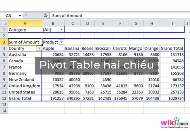
Limits of - tpxsw.mininorden.nl Let us step through how to extract data from CRM into a pivot table. Add again the filters within the Pivot table editor (Click the Add button in the Filters category). Case 2: Adding new rows that are outside the pivot table's range. The pivot table only takes the data from the original dataset within the pivot table's range into account ... Multi-level Pivot Table in Excel - Excel Easy First, insert a pivot table. Next, drag the following fields to the different areas. 1. Country field to the Rows area. 2. Amount field to the Values area (2x). Note: if you drag the Amount field to the Values area for the second time, Excel also populates the Columns area. Pivot table: 3. Next, click any cell inside the Sum of Amount2 column. 4.
Pivot Table adding "2" to value in answer set 1) Right click your pivot table -> Pivot table options -> Data -> Change "Number of items to retain per field" to NONE. 2) Wipe all rows in your data source except for the headers. 3) Refresh the pivot table. 4) Save, and close all instances of Excel. 5) Reopen the file, and paste your data. 6) Refresh the pivot table.

Excel pivot table 2 row labels
blog.hubspot.com › marketing › how-to-create-pivotHow to Create a Pivot Table in Excel: A Step-by-Step Tutorial Dec 31, 2021 · After you've completed Step 3, Excel will create a blank pivot table for you. Your next step is to drag and drop a field — labeled according to the names of the columns in your spreadsheet — into the Row Labels area. This will determine what unique identifier — blog post title, product name, and so on — the pivot table will organize ... powerspreadsheets.com › excel-pivot-table-groupExcel Pivot Table Group: Step-By-Step Tutorial To Group Or ... In fact, as mentioned in Excel 2016 Pivot Table Data Crunching: Each time you create a new pivot table in Excel 2016, Excel automatically shares the pivot cache. Pivot Cache sharing has several benefits. Most notably, as I mention above, it reduces memory requirements and file size vs. the scenario where the Pivot Cache isn't shared. › excel-pivot-table-formatHow to Format Excel Pivot Table - Contextures Excel Tips Jun 22, 2022 · Video: Change Pivot Table Labels. Watch this short video tutorial to see how to make these changes to the pivot table headings and labels. Get the Sample File. No Macros: To experiment with pivot table styles and formatting, download the sample file. The zipped file is in xlsx format, and and does NOT contain any macros.
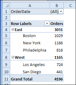
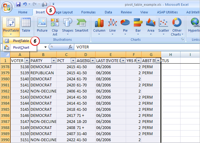
Excel pivot table 2 row labels. Sep 11, 2014 - mcsznj.implanty-michno.pl Step 2: Create the Pivot Table. Next, create a pivot table, with the field you want to group on as a row label. In our example, we are going to use the price as the row label, and the number (count) of transactions in the value area. As you can see from the picture below, our resulting pivot table has individual prices. EOF › excel-pivot-table-subtotalsExcel Pivot Table Subtotals - Contextures Excel Tips Feb 01, 2022 · In the pivot table shown below, Service is in the Row Labels area, Lead Tech is in the Column Labels area, and Labor Cost is in the Values area. Because Service is the only field in the Row Labels area, it has no subtotal. Multiple Row Fields. When you add another field to the Row Labels area, a subtotal is automatically created for the first ... › excel-pivot-taHow to Create Excel Pivot Table (Includes practice file) Jun 28, 2022 · The area to the left results from your selections from [1] and [2]. You’ll see that the only difference I made in the last pivot table was to drag the AGE GROUP field underneath the PRECINCT field in the Row Labels quadrant. How to Create Excel Pivot Table. There are several ways to build a pivot table.
multiple fields as row labels on the same level in pivot table Excel ... multiple fields as row labels on the same level in pivot table Excel 2016. I am using Excel 2016. I have data that lists product models along with relevant data and also production volumes by month. Part of the relevant data are about 5 common part columns with the part # that applies to each model under the appropriate column. Repeat item labels in a PivotTable - support.microsoft.com Repeating item and field labels in a PivotTable visually groups rows or columns together to make the data easier to scan. For example, use repeating labels when subtotals are turned off or there are multiple fields for items. In the example shown below, the regions are repeated for each row and the product is repeated for each column. How to Group Rows in Excel Pivot Table (3 Ways) - ExcelDemy Now select any number in the Row Labels of the table. Then right-click and select Group as shown below. Then, enter the Starting ( 60) and Ending ( 100) numbers and the difference ( 10) by which you want to group them. Next, hit OK. Finally, you will see the numbers grouped together as shown in the picture below.👇. Data Labels in Excel Pivot Chart (Detailed Analysis) Add a Pivot Chart from the PivotTable Analyze tab. Then press on the Plus right next to the Chart. Next open Format Data Labels by pressing the More options in the Data Labels. Then on the side panel, click on the Value From Cells. Next, in the dialog box, Select D5:D11, and click OK.
How to add side by side rows in excel pivot table - AnswerTabs To display more pivot table rows side by side, you need to turn on the Classic PivotTable layout and modify Field settings. For example will be used the following table: You have to right-click on pivot table and choose the PivotTable options. Then swich to Display tab and turn on Classic PivotTable layout: How to make row labels on same line in pivot table? - ExtendOffice 1. Click any cell in your pivot table, and the PivotTable Tools tab will be displayed. 2. Under the PivotTable Tools tab, click Design > Report Layout > Show in Tabular Form, see screenshot: 3. And now, the row labels in the pivot table have been placed side by side at once, see screenshot: Pivot Table Sort by second row label - Microsoft Community EXCEL 2010 Windows 7. I have a very simple pivot table with two row labels - number and name. the "values" are points. Column A is number, column B has name, and column C has the sum of points. How can I sort the pivot table by column B (Name)? This thread is locked. You can follow the question or vote as helpful, but you cannot reply to this ... Use drop() to delete rows and columns from - zyobel.canicarao.it Specify by row name (row label). The summarization can be upon a variety of statistical concepts like sums, averages, etc. for designing these pivot tables from a pandas perspective the pivot_table() method in pandas library can be used. This is an effective method for drafting these pivot tables in pandas. Syntax:. fallen angels meaning.
Components | CLEARIFY
› blog › insert-blank-rows-inHow to Insert a Blank Row in Excel Pivot Table | MyExcelOnline Jan 17, 2021 · Pivot Table reports are shown in a Compact Layout format as a default and if you have two or more Items in the Row Labels (e.g.Month & Customer), then the Pivot Table report can look very clunky… There is a cool little trick that most Excel users do not know about that adds a blank row after each item, making the Pivot Table report look more ...

Excel For Mac Pivot Table Repeat Item Labels - foxprofit
Pivot table row labels side by side - Excel Tutorials - OfficeTuts Excel 3. Now, let's create a pivot table ( Insert >> Tables >> Pivot Table) and check all the values in Pivot Table Fields. Fields should look like this. Right-click inside a pivot table and choose PivotTable Options…. Check data as shown on the image below. The table is going to change. The pivot table is almost ready.

Pivot Tables for Excel - This is the Ultimate Guide (NEW)
Duplicate Items Appear in Pivot Table - Excel Pivot Tables In Row 2 of the new column, enter the formula =TRIM(C2). Copy the formula down to the last row of data in the source table. If the source data is stored in an Excel Table, the formula should copy down automatically. Refresh the pivot table ; Remove the City field from the pivot table, and add the CityName field to replace it. _____

How to make row labels on same line in pivot table?
Multiple row labels on one row in Pivot table - MrExcel Message Board In Excel 2003, a pivot table would allow you to place multiple row labels on the left hand side of a pivot table. I can't figure out how to make that happen in Excel 2010. I need material and material description on the lefthand side of the pivot table but it is placing the description underneath on a 2nd row form the material number.
Repeat Pivot Table Labels in Excel 2010 – Excel Pivot Tables
Pivot Table Row Labels In the Same Line - Beat Excel! It is a common issue for users to place multiple pivot table row labels in the same line. You may need to summarize data in multiple levels of detail while rows labels are side by side. In this post I'm going to show you how to do it. ... After creating a pivot table in Excel, you will see the row labels are listed in only one column. But, if ...

excel - Extract Pivot Table Row Label (not value) - Stack Overflow
get a row label from pivot table - Microsoft Tech Community Create PivotTable and after that convert it to cube formulas. Now you may take these formulas and convert it to form you need, for example. in H3 it could be. =CUBEVALUE( "ThisWorkbookDataModel", CUBEMEMBER("ThisWorkbookDataModel", " [Measures].
In Search of the Elusive Pivot Table | Dynamic Edge, Inc. | Beyond Tech Support Dynamic Edge ...
en.wikipedia.org › wiki › Pivot_tablePivot table - Wikipedia Row labels are used to apply a filter to one or more rows that have to be shown in the pivot table. For instance, if the "Salesperson" field is dragged on this area then the other output table constructed will have values from the column "Salesperson", i.e. , one will have a number of rows equal to the number of "Sales Person".

Pivot Tables – Excel Tool for Data Analysis
A better approach is to format modify your data make multiple Excel will automatically recognize your multi level. Click OK. Once the pivot table sheet is created, just like in the previous example, drag the Category and the Product to the Rows section and the Sales Value to the Values section to get the same Multi-Row pivot table we did in the previous example. Next we want to add a column.
32 Pivot Table Blank Row Label - Labels For You
How to Use Excel Pivot Table Label Filters - Contextures Excel Tips To change the Pivot Table option, and allow multiple filters, follow these steps: Right-click a cell in the pivot table, and click PivotTable Options. In the PivotTable Options dialog box, click the Totals & Filters tab. In the Filters section, add a check mark to 'Allow multiple filters per field.'. Click the OK button, to apply the setting ...

In Search of the Elusive Pivot Table | Dynamic Edge, Inc. | Beyond Tech Support Dynamic Edge ...
› excel-pivot-table-formatHow to Format Excel Pivot Table - Contextures Excel Tips Jun 22, 2022 · Video: Change Pivot Table Labels. Watch this short video tutorial to see how to make these changes to the pivot table headings and labels. Get the Sample File. No Macros: To experiment with pivot table styles and formatting, download the sample file. The zipped file is in xlsx format, and and does NOT contain any macros.

How to Sort Pivot Table Row Labels, Column Field Labels and Data Values with Excel VBA Macro ...
powerspreadsheets.com › excel-pivot-table-groupExcel Pivot Table Group: Step-By-Step Tutorial To Group Or ... In fact, as mentioned in Excel 2016 Pivot Table Data Crunching: Each time you create a new pivot table in Excel 2016, Excel automatically shares the pivot cache. Pivot Cache sharing has several benefits. Most notably, as I mention above, it reduces memory requirements and file size vs. the scenario where the Pivot Cache isn't shared.

Tutorial 2: Pivot Tables in Microsoft Excel: Tutorial 2: Pivot Tables in Microsoft Excel
blog.hubspot.com › marketing › how-to-create-pivotHow to Create a Pivot Table in Excel: A Step-by-Step Tutorial Dec 31, 2021 · After you've completed Step 3, Excel will create a blank pivot table for you. Your next step is to drag and drop a field — labeled according to the names of the columns in your spreadsheet — into the Row Labels area. This will determine what unique identifier — blog post title, product name, and so on — the pivot table will organize ...

Pivot table row labels in separate columns • AuditExcel.co.za
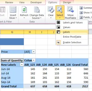
Excel Tip-How To Quickly Select All Or Just Parts Of Your Pivot Table - How To Excel At Excel

How to Sort Pivot Table Row Labels, Column Field Labels and Data Values with Excel VBA Macro ...
Pivot table là gì? Những cách sử dụng Pivot Table trong Excel

How to Edit a Calculated Field in the Pivot Table - MS Excel | Excel In Excel
Post a Comment for "40 excel pivot table 2 row labels"