44 scatter chart in excel with labels
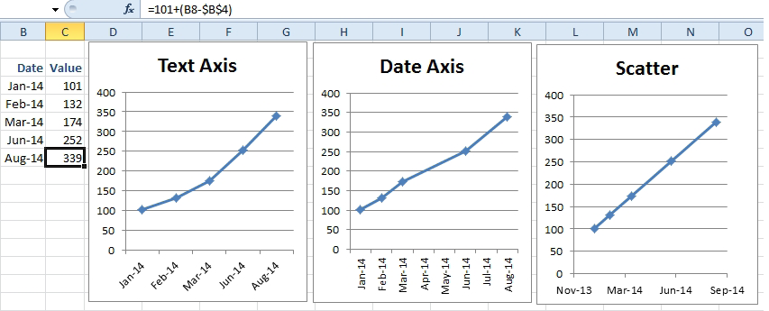
Labeling X-Y Scatter Plots (Microsoft Excel) Just enter "Age" (including the quotation marks) for the Custom format for the cell. Then format the chart to display the label for X or Y value. When you do this, the X-axis values of the chart will probably all changed to whatever the format name is (i.e., Age). However, after formatting the X-axis to Number (with no digits after the decimal ... How to add axis label to chart in Excel? - ExtendOffice Navigate to Chart Tools Layout tab, and then click Axis Titles, see screenshot: 3.
Excel Chart Vertical Axis Text Labels - My Online Training Hub So all we need to do is get that bar chart into our line chart, align the labels to the line chart and then hide the bars. We’ll do this with a dummy series: Copy cells G4:H10 (note row 5 is intentionally blank) > CTRL+C to copy the cells > select the chart > CTRL+V to paste the dummy data into the chart.

Scatter chart in excel with labels
Hover labels on scatterplot points - Excel Help Forum Hi Everyone, I am hoping someone can point me in the right direction on a challenge I am trying to solve. I have data on an xy scatterplot and would like to be able to move by mouse over the points and have a label show up for each point showing the X,Y value of the point and also text from a comment cell. I know excel has these hover labels but i cant seem to find a way to edit them. How to Make a Scatter Plot in Excel (XY Chart) - Trump Excel This can be done by using a Scatter chart in Excel. For example, if you have the Height (X value) and Weight (Y Value) data for 20 students, you can plot this in a scatter chart and it will show you how the data is related. ... Do add the data labels to the scatter chart, select the chart, click on the plus icon on the right, and then check the ... Creating Scatter Plot with Marker Labels - Microsoft Community Right click any data point and click 'Add data labels and Excel will pick one of the columns you used to create the chart. Right click one of these data labels and click 'Format data labels' and in the context menu that pops up select 'Value from cells' and select the column of names and click OK.
Scatter chart in excel with labels. How to use a macro to add labels to data points in an xy scatter chart ... The labels and values must be laid out in exactly the format described in this article. (The upper-left cell does not have to be cell A1.) To attach text labels to data points in an xy (scatter) chart, follow these steps: On the worksheet that contains the sample data, select the cell range B1:C6. How do I set labels for each point of a scatter chart? Click one of the data points on the chart. Chart Tools. Layout contextual tab. Labels group. Click on the drop down arrow to the right of:- Data Labels Make your choice. If my comments have helped please vote as helpful. Thanks. Report abuse Was this reply helpful? Replies (2) Scatter chart horizontal axis labels | MrExcel Message Board Apr 26, 2011. #3. Use a Line chart (rather than a XY Scatter chart) and you can have any text in the X values. If you must use a XY Chart, you will have to simulate the effect. Add a dummy series which will have all y values as zero. Then, add data labels for this new series with the desired labels. Locate the data labels below the data points ... XY scatter chart in Excel. Custom labels for the points - YouTube 00:00 XY/ Scatter charts- Useful but a bit harder to setup 00:22 Compare Revenue growth % to Gross Margin %00:40 First column of data is the horizontal/ x ax...
Scatter Plots in Excel with Data Labels Select "Chart Design" from the ribbon then "Add Chart Element" Then "Data Labels". We then need to Select again and choose "More Data Label Options" i.e. the last option in the menu. This will... Custom Axis Labels and Gridlines in an Excel Chart Jul 23, 2013 · Here is the XY Scatter chart of the First (blue) and Second (orange) data sets. I guess it’s a question mark symbolizing the confusion expressed by the original questioner. ... Select the horizontal dummy series and add data labels. In Excel 2007-2010, go to the Chart Tools > Layout tab > Data Labels > More Data Label Options. In Excel 2013 ... Excel scatter chart using text name - Access-Excel.Tips Since Excel allows different chart types to be displayed in one chart, we are going to create a mix of bar chart (column chart) and scatter chart. Scatter chart is used to display the actual data point, while bar chart is to display Grade labels. - Create scatter chart for Range B20:C31 (Series 1) excel - How to getting text labels to show up in scatter chart - Stack ... How to getting text labels to show up in scatter chart. I want text labels for my scatter plot that is connected with points in the graph. my data is like this. The chart removes the labels and places numbers. How do I get the text labels back?
Add a Horizontal Line to an Excel Chart - Peltier Tech Sep 11, 2018 · As with the XY Scatter chart in the first example, we need to figure out what to use for X and Y values for the line we’re going to add. The Y values are easy, but the X values require a little understanding of how Excel’s category axes work. ... To begin with, the range I used to populate the chart had the letters in the first column, and ... How to Make a Scatter Plot in Excel and Present Your Data May 17, 2021 · Add Labels to Scatter Plot Excel Data Points. You can label the data points in the X and Y chart in Microsoft Excel by following these steps: Click on any blank space of the chart and then select the Chart Elements (looks like a plus icon). Then select the Data Labels and click on the black arrow to open More Options. Create an X Y Scatter Chart with Data Labels - YouTube How to create an X Y Scatter Chart with Data Label. There isn't a function to do it explicitly in Excel, but it can be done with a macro. The Microsoft Kno... How to use a macro to add labels to data points in an xy scatter chart ... In Microsoft Office Excel 2007, follow these steps: Click the Insert tab, click Scatter in the Charts group, and then select a type. On the Design tab, click Move Chart in the Location group, click New sheet , and then click OK. Press ALT+F11 to start the Visual Basic Editor. On the Insert menu, click Module.
3d scatter plot for MS Excel
How to find, highlight and label a data point in Excel scatter plot To let your users know which exactly data point is highlighted in your scatter chart, you can add a label to it. Here's how: Click on the highlighted data point to select it. Click the Chart Elements button. Select the Data Labels box and choose where to position the label.

Scatter Chart in Microsoft Excel
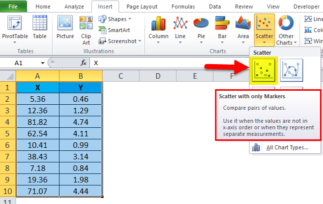
how to make a scatter plot in Excel - storytelling with data Highlight the two columns you want to include in your scatter plot. Then, go to the " Insert " tab of your Excel menu bar and click on the scatter plot icon in the " Recommended Charts " area of your ribbon. Select "Scatter" from the options in the "Recommended Charts" section of your ribbon.

Excel Charts | Real Statistics Using Excel
How to Make a Scatter Plot in Excel and Present Your Data Add Labels to Scatter Plot Excel Data Points. You can label the data points in the X and Y chart in Microsoft Excel by following these steps: Click on any blank space of the chart and then select the Chart Elements (looks like a plus icon). Then select the Data Labels and click on the black arrow to open More Options.
Excel Scatter Chart - Super User
How to Create a Quadrant Chart in Excel - Automate Excel Click the " Insert Scatter (X, Y) or Bubble Chart. " Choose " Scatter. " Step #2: Add the values to the chart. Once the empty chart appears, add the values from the table with your actual data. Right-click on the chart area and choose " Select Data ." Another menu will come up. Under Legend Entries (Series), click the " Add " button.
Scatter Chart in Excel (Examples) | How To Create Scatter Chart in Excel?
Scatter Plot Chart in Excel (Examples) | How To Create Scatter ... - EDUCBA Step 1: Select the data. Step 2: Go to Insert > Chart > Scatter Chart > Click on the first chart. Step 3: This will create the scatter diagram. Step 4: Add the axis titles, increase the size of the bubble and Change the chart title as we have discussed in the above example. Step 5: We can add a trend line to it.
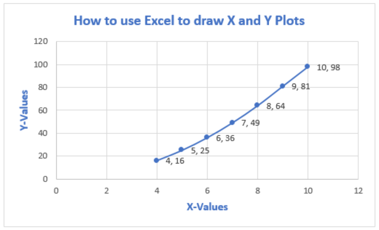
How To Plot X Vs Y Data Points In Excel | Excelchat
Add or remove data labels in a chart - support.microsoft.com Click the data series or chart. To label one data point, after clicking the series, click that data point. In the upper right corner, next to the chart, click Add Chart Element > Data Labels. To change the location, click the arrow, and choose an option. If you want to show your data label inside a text bubble shape, click Data Callout.
X-Y Chart (Excel 2010) - Step 2 Construct a Scatter Chart with Labels - YouTube
Excel: labels on a scatter chart, read from array - Stack Overflow Excel: labels on a scatter chart, read from array Ask Question 0 Here I have a chart I did a right-click -> "Add labels" , and it read them from my a (H/C) row. Basically, I want it to read label values from the CO2/CH4 row instead, so they would be 0,0.5,1,2,5,10 instead.

Scatter Chart in Excel (Examples) | How To Create Scatter Chart in Excel?
How to display text labels in the X-axis of scatter chart in Excel? Display text labels in X-axis of scatter chart Actually, there is no way that can display text labels in the X-axis of scatter chart in Excel, but we can create a line chart and make it look like a scatter chart. 1. Select the data you use, and click Insert > Insert Line & Area Chart > Line with Markers to select a line chart. See screenshot: 2.
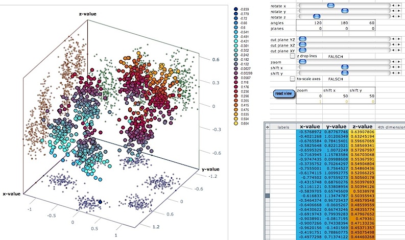
3d scatter plot for MS Excel
Wrap category names (Y axis labels) of a scatter chart? The labels are the standard axes labels and you have very limited control over their layout. You can add line feeds to wrap the text by adding ALT+ENTER to the text in the cells. If you want full control you will need to create your own textboxes to use as labelling. Register To Reply Bookmarks
Excel: Scatter Charts are Versatile But Require a Different Workflow - Excel Articles
How to Find, Highlight, and Label a Data Point in Excel Scatter Plot? By default, the data labels are the y-coordinates. Step 3: Right-click on any of the data labels. A drop-down appears. Click on the Format Data Labels… option. Step 4: Format Data Labels dialogue box appears. Under the Label Options, check the box Value from Cells . Step 5: Data Label Range dialogue-box appears.

Multiple Series in One Excel Chart - Peltier Tech Blog
How to Change Excel Chart Data Labels to Custom Values? May 05, 2010 · When you “add data labels” to a chart series, excel can show either “category” , “series” or “data point values” as data labels. But what if you want to have a data label that is altogether different, like this: ... Hi I am preparing a X-Y scatter chart. Now when i hover over the scatter points, a hover label appears which shows ...

Risk matrix chart in Power BI - Microsoft Power BI Community
How to Add Labels to Scatterplot Points in Excel - Statology Step 3: Add Labels to Points. Next, click anywhere on the chart until a green plus (+) sign appears in the top right corner. Then click Data Labels, then click More Options…. In the Format Data Labels window that appears on the right of the screen, uncheck the box next to Y Value and check the box next to Value From Cells.
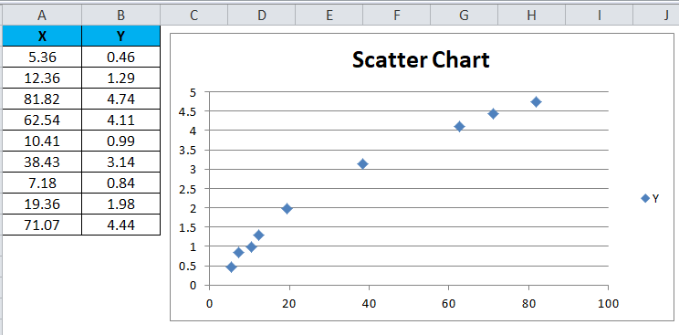
Scatter Chart in Excel (Examples) | How To Create Scatter Chart in Excel?
Scatter Plot with Text Labels on X-axis : excel For example, consider a formula like this: =IF (XLOOKUP (A1,B:B,C:C)>5,XLOOKUP (A1,B:B,C:C)+3,XLOOKUP (A1,B:B,C:C)-2) So basically a lookup or something else with a bit of complexity, is referenced multiple times. Now this isn't too bad in this example, but you can often have instances where you need to call the same sub-function multiple times ...

Scatter Chart in Excel
How to display text labels in the X-axis of scatter chart in Excel? Display text labels in X-axis of scatter chart. Actually, there is no way that can display text labels in the X-axis of scatter chart in Excel, but we can create a line chart and make it look like a scatter chart. 1. Select the data you use, and click Insert > Insert Line & Area Chart > Line with Markers to select a line chart. See screenshot:
Combine pie and xy scatter charts - Advanced Excel Charting Example
How To Create Scatter Chart in Excel? - EDUCBA To apply the scatter chart by using the above figure, follow the below-mentioned steps as follows. Step 1 - First, select the X and Y columns as shown below. Step 2 - Go to the Insert menu and select the Scatter Chart. Step 3 - Click on the down arrow so that we will get the list of scatter chart list which is shown below.
Post a Comment for "44 scatter chart in excel with labels"